OccBin Toolbox  V2.0

A MATLAB/Dynare toolkit for solving dynamic models with occasionally binding constraints easily — updated for Dynare 6.5 and Dynare 7.0.

Luca Guerrieri  ·  Matteo Iacoviello

⇓  Download Toolbox View Walkthrough →

Requires Dynare 6.5 or 7.0  |  MATLAB R2026a  |  macOS ARM64 verified

📰

Published paper

OccBin: A Toolkit to Solve Models with Occasionally Binding Constraints Easily

Luca Guerrieri & Matteo Iacoviello  —  Journal of Monetary Economics, Vol. 70 (2015), pp. 22–38  ·  doi:10.1016/j.jmoneco.2014.08.005

Piecewise-linear solutions for constrained models

OccBin solves DSGE models in which one or two constraints bind occasionally — zero lower bounds, borrowing limits, irreversibility — without requiring global methods or perfect-foresight solvers. The algorithm pieces together regime-specific linear solutions, iterating until the sequence of binding periods is consistent.

🔗

One Constraint

Solves models that switch between a reference regime and one alternative regime, such as a zero lower bound on the nominal interest rate or an irreversibility constraint on investment.

Two Constraints

Extends the algorithm to models with two simultaneously active constraints — four possible regime combinations — using solve_two_constraints_add_violvecbool.

📄

Any Dynare Model

Works with any model written as a pair of standard Dynare .mod files: one for the unconstrained regime and one for the binding regime. Variables and parameters must be declared in the same order in both files.

What you need before you start

Running your first example

Three steps get you from a fresh download to a working IRF chart.

1

Set the Dynare and toolkit path

From the toolbox root directory, run the path script that matches your Dynare installation. Edit the script once to point to your local Dynare directory; after that it can be called from any subfolder.

% For Dynare 6.5:
setpathdynare6_5

% For Dynare 7.0:
setpathdynare7
2

Navigate to a model directory

Each example lives in its own subfolder. Change into the folder for the example you want to run.

cd 'path/to/occbin/model_irrcap'   % irreversible investment example
% or
cd 'path/to/occbin/model_newkeynesian'  % ZLB example
3

Run the entry-point script

Each model directory ships a runsim_*.m script that sets up the shock sequence, calls the solver, unpacks results, and plots IRFs.

runsim_irrcap          % irreversible investment
runsim_newkeynesian    % New Keynesian ZLB
runsim_borrcon         % borrowing constraint
runsim_dnk             % DNK ZLB + government spending
runsim_cgg             % CGG inertial Taylor rule + ZLB
runsim_smetswouters    % Smets-Wouters 2007 + ZLB
Automated testing: Run run_all_tests.m from the root to execute all nine examples and see PASS/FAIL for each — useful after modifying toolkit files.

Adapting the toolkit to a new model

To apply OccBin to your own model, you need two Dynare .mod files and a runsim_*.m script. Follow these conventions:

Key toolbox functions

solve_one_constraint — one occasionally binding constraint

[zdatalinear_, zdatapiecewise_, zdatass_, oobase_, Mbase_,
 Mstar_, oostar_, optionsbase_, optionsstar_, check,
 newviolvecbool_, relaxconstraint_] =
solve_one_constraint(modnam, modnamstar,
  constraint, constraint_relax,
  shockssequence, irfshock, nperiods, maxiter, init);

Inputs

ArgumentTypeDescription
modnamstring Name of the .mod file for the reference regime (constraint not binding). Omit the .mod extension.
modnamstarstring Name of the .mod file for the alternative regime (constraint binding). Omit the .mod extension.
constraintstring Expression (in contemporaneous variables, deviations from steady state) that evaluates to true when the solution should switch to the alternative regime. Example: 'i<log(PHII)'.
constraint_relaxstring Expression that evaluates to true when the solution returns to the reference regime. Example: 'lambdak<0'.
shockssequenceT × nshocks matrix Sequence of unforeseen shocks. Each row is one period; each column corresponds to one varexo.
irfshockstring or char array Label(s) of the innovation(s) for IRFs — must match a varexo name in the .mod file.
nperiodsinteger Simulation horizon. Must be long enough for the model to return to the reference regime by the end of the window.
maxiterinteger (default 20) Maximum number of fixed-point iterations. Increase if check = -1.
initvector (optional) Initial state vector in deviation from steady state. Default is steady state. Ordering follows the .mod definition order.

Outputs

OutputDescription
zdatalinear_ nperiods × nvars array. Paths for all endogenous variables ignoring the constraint (pure linear solution), in deviation from steady state.
zdatapiecewise_ nperiods × nvars array. Paths satisfying the constraint (OccBin piecewise-linear solution), in deviation from steady state.
zdatass_ Vector of steady-state values, following .mod definition order.
oobase_, Mbase_ Dynare output structures for the reference model.
Mstar_, oostar_, optionsbase_, optionsstar_ Dynare structures for the alternative regime model.
check 0 if the algorithm converged; -1 if it did not (increase maxiter or nperiods).
newviolvecbool_, relaxconstraint_ Boolean vectors indicating, period by period, when the constraint binds and when the relax condition holds.

solve_two_constraints_add_violvecbool — two occasionally binding constraints

[zdatalinear_, zdatapiecewise_, zdatass_, oo00_, M00_,
 violvecbool_last_shock, M10_, M01_, M11_,
 options00_, ..., check] =
solve_two_constraints_add_violvecbool(
  modnam_00, modnam_10, modnam_01, modnam_11,
  constraint1, constraint2,
  constraint_relax1, constraint_relax2,
  shockssequence, irfshock, nperiods,
  curb_retrench, maxiter, init);

Model files (four regimes)

ArgumentRegime
modnam_00Neither constraint binds (reference regime)
modnam_10Only constraint 1 binds
modnam_01Only constraint 2 binds
modnam_11Both constraints bind simultaneously

All other inputs mirror solve_one_constraint, with the addition of curb_retrench: a scalar (0 or 1, default 0). When set to 1, the regime-update step slows to a Gauss-Jacobi scheme — useful when the default full update does not converge.

Important notes

Writing the constraint string. Variables in constraint and constraint_relax refer to deviations from steady state, not levels. For example, if the model constraint is it ≥ log(φ · Iss), the linearized form simplifies to ĩt < log(φ), so the string is 'i<log(PHII)'. Parameters and numerical constants are evaluated in the MATLAB workspace.
Contemporaneous variables only. Both constraint and constraint_relax may only involve contemporaneous endogenous variables. Lagged or leaded variables are not permitted in these expressions; use auxiliary variable definitions in the .mod file to work around this if needed.
Steady state and alternative regimes. You do not need to specify the steady state of any alternative model. All regimes are approximated around the steady state of the reference model. Parameter values set in the alternative model's .mod file are ignored at runtime — only the reference model's parameter values are used.

Nine worked examples

Three examples replicate the models in the paper; six additional examples cover richer constraint structures, alternative solvers, and larger-scale models.

Paper examples

model_irrcap/

RBC model with irreversible investment: investment cannot fall below a fraction PHII of its steady-state level. Entry point: runsim_irrcap.m. See the full walkthrough below.

model_newkeynesian/

Fuhrer-Violante New Keynesian model with a zero lower bound on the nominal interest rate. The notional rate rnot switches regime when it goes negative. Entry point: runsim_newkeynesian.m.

model_borrcon/

Small open-economy model with an occasionally binding borrowing constraint: Bt = mYt. Demonstrates constraints expressed in terms of a multiplier. Entry point: runsim_borrcon.m.

Additional examples

model_irrcap_twoconstraints/

RBC model with two simultaneous constraints: irreversible investment (IRR) and no-negative-investment (INEG). Uses four .mod files — one per regime combination. Entry points: runsim_irrcap_two_constraints.m and runsim_irrcap_two_constraints_computepolicy.m (derives nonlinear policy functions).

model_irrcap_dynoccbin/

The irreversible-investment RBC model reimplemented with Dynare 7's built-in OccBin solver (occbin_constraints, occbin_setup, occbin_solver). A single dynrbc_occbin.mod replaces the two-file approach. Outputs match model_irrcap to machine precision. Requires Dynare 7.0. Entry point: runsim_irrcap_dynoccbin.m.

model_cgg/

Clarida-Gali-Gertler (1999) model with an inertial Taylor rule subject to the zero lower bound. The notional rate rnot triggers regime switching. Entry point: runsim_cgg.m.

model_smetswouters/

Smets-Wouters (AER, 2007) US model extended with a zero lower bound. Parameters are set at their pre-estimation initial values to skip the estimation step. Entry point: runsim_smetswouters.m.

model_dnk/

Dynamic New Keynesian model with zero lower bound and government spending. Shows how to use a single external parameter file (paramfile_dnk.m) and how to compute IRFs conditional on different baseline paths. Entry point: runsim_dnk.m.

run_all_tests.m

Automated test runner that executes all nine runsim_*.m scripts and reports PASS/FAIL for each. All nine pass on both Dynare 6.5 and 7.0. Run after setpathdynare6_5 or setpathdynare7.

Irreversible Investment — model_irrcap

This example, the first in the paper, applies OccBin to an RBC model in which investment cannot fall below a fixed fraction of its steady-state level. It illustrates the complete workflow: two .mod files, a constraint string, a shock sequence, and the resulting IRF chart.

OccBin IRF chart: piecewise-linear vs. linear responses in the irreversible-investment RBC model
Figure: Piecewise-linear vs. linear IRFs
Responses to a positive then negative TFP shock sequence

Consumption, capital, investment, TFP, multiplier — 100 periods.

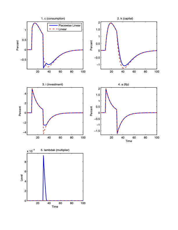
Impulse responses to a positive TFP shock at period 10 and a negative shock at period 30. Blue: piecewise-linear (OccBin). Red: linear (ignoring constraint). When investment is forced to its floor, the piecewise solution diverges sharply from the linear one.

1

The model and its constraint

The model is a standard RBC model with a capital adjustment cost (PSI) and a Lagrange multiplier lambdak on the investment floor. In the reference regime (constraint not binding), the multiplier is zero: lambdak = 0. In the alternative regime (constraint binding), investment is pegged to its lower bound: i = log(PHII · ISS).

The occasionally binding constraint is It ≥ φ · Iss, or in log-deviation form: ĩt ≥ log(φ). The constraint is violated — and regime switches — when the linear solution produces investment below this floor.

Variables in both .mod files:

VariableDescription
aTotal factor productivity (log)
cConsumption (log)
iInvestment (log)
kCapital (log, end of period)
kprevLagged capital, defined as k(-1)
lambdakLagrange multiplier on the investment floor
2

The two .mod files

The reference file dynrbc.mod sets lambdak = 0 (equation 4 below). The alternative file dynrbcirr_i.mod is an exact replica except that equation 4 is replaced by i = log(PHII · ziss), enforcing the investment floor. All other equations and the parameter list are identical.

// dynrbc.mod — reference regime (constraint not binding)
var a, c, i, k, kprev, lambdak;
varexo erra;
parameters ALPHA, DELTAK, BETA, GAMMAC, RHOA, PHII, PHIK, PSI, PSINEG, ISS, KSS;

model;
// 1. Euler equation (capital)
-exp(c)^(-GAMMAC)*(1+2*PSI*(exp(k)/exp(k(-1))-1)/exp(k(-1)))
+ BETA*exp(c(1))^(-GAMMAC)*((1-DELTAK)
  -2*PSI*(exp(k(1))/exp(k)-1)*(-exp(k(1))/exp(k)^2)
  +ALPHA*exp(a(1))*exp(k)^(ALPHA-1))
  = -lambdak + BETA*(1-DELTAK+PHIK)*lambdak(1);

// 2. Resource constraint
exp(c)+exp(k)-(1-DELTAK)*exp(k(-1))+PSI*(exp(k)/exp(k(-1))-1)^2
  = exp(a)*exp(k(-1))^ALPHA;

// 3. Investment definition
exp(i) = exp(k)-(1-DELTAK)*exp(k(-1));

// 4. Reference regime: multiplier is zero
lambdak = 0;

// 5. TFP process
a = RHOA*a(-1) + erra;

kprev = k(-1);
end;
// dynrbcirr_i.mod — alternative regime (investment at floor)
// Identical to dynrbc.mod except equation 4:

// 4. Alternative regime: investment is pinned to its lower bound
i = log(PHII*ziss);
Key rule: every var, varexo, and parameters declaration must appear in the same order in both files. Only the binding-regime equation changes.
3

Parameter values

Parameter values are set in paramfile_dynrbc.m, loaded by the Dynare steady-state file at parse time.

BETA   = 0.96;    % discount factor
ALPHA  = 0.33;    % capital share
DELTAK = 0.10;    % depreciation rate
GAMMAC = 2;       % inverse elasticity of substitution
RHOA   = 0.9;     % TFP persistence
PHII   = 0.975;   % investment floor as fraction of I_ss
PSI    = 0;       % capital adjustment cost (zero here)

The toolkit computes steady-state capital and investment from these primitives: Kss = ((1/β − 1 + δ) / α)1/(α−1),  Iss = δ Kss.

4

Setting up and calling the solver

The script runsim_irrcap.m specifies the shock sequence and calls solve_one_constraint. Here, a positive 2% TFP shock hits at period 10 and a symmetric negative shock at period 30, over a 100-period horizon.

clear
global M_ oo_

modnam     = 'dynrbc';        % reference regime .mod file
modnamstar = 'dynrbcirr_i';   % alternative regime .mod file

% Constraint string (in deviation from steady state)
constraint       = 'i<log(PHII)';   % switch to alt. regime when i hits floor
constraint_relax = 'lambdak<0';     % return to ref. regime when multiplier goes negative

irfshock = char('erra');       % TFP innovation

shockssequence = zeros(60,1);
shockssequence(10) =  0.02;      % positive shock at period 10
shockssequence(30) = -0.02;      % negative shock at period 30

nperiods = 100;
maxiter  = 10;

[zdatalinear, zdatapiecewise, zdatass, oobase_, Mbase_] = ...
  solve_one_constraint(modnam, modnamstar, ...
    constraint, constraint_relax, ...
    shockssequence, irfshock, nperiods, maxiter);
5

Unpacking and plotting results

After the solver returns, the script unpacks the output arrays into named workspace variables using a loop over the endogenous variable list, then calls makechart to plot piecewise-linear and linear paths side by side.

% Unpack all endogenous variables from the output matrices
for i = 1:Mbase_.endo_nbr
  eval([Mbase_.endo_names{i}, '_l = zdatalinear(:,i);']);
  eval([Mbase_.endo_names{i}, '_p = zdatapiecewise(:,i);']);
  eval([Mbase_.endo_names{i}, '_ss = zdatass(i);']);
end

% Build chart inputs
titlelist  = char('c (consumption)','k (capital)','i (investment)', ...
                   'a (tfp)','lambdak (multiplier)');
ylabels    = char('Percent','Percent','Percent','Percent','Level');
legendlist = cellstr(char('Piecewise Linear','Linear'));

line1 = 100*[c_p, k_p, i_p, a_p, (lambdak_p + lambdak_ss)/100];
line2 = 100*[c_l, k_l, i_l, a_l, (lambdak_l + lambdak_ss)/100];

makechart(titlelist, legendlist, '', ylabels, line1, line2)
What to look for: When the negative shock at period 30 drives investment to its floor, the piecewise-linear path for consumption and capital diverges from the unconstrained linear path. The multiplier lambdak turns positive during the binding episodes, signalling that the constraint is active.

Download the toolbox

All source code, model examples, and pre-generated output files are packaged in a single zip archive.

⇓  occbin_06162026.zip

Contains: toolkit_files/  ·  nine model examples  ·  Dynare 6.5 & 7.0 compatible